Currency Depreciation: No one size fits all

• A devaluation or depreciation of a currency (under a fixed or floating regime, respectively) is expected to improve a country’s trade balance.
• The J-curve effect states that a country’s trade balance will initially worsen in the short run after the devaluation and will improve after a certain lag that will reflect itself in the long run.
• Deals with the brief period immediately following devaluation (or depreciation) in which contracts were negotiated prior to the change falls due.
• The results of the econometric analysis empirically established that for the Developed and Developing countries there exists a positive statistically significant relationship at 1%, between Exchange Rate Devaluation (or depreciation) and BOT and for the LDCs, there exists a negative but statistically significant relationship at 1%.

The “competitive devaluation” through which a country could improve its trading position by weakening its currency has long captured the attention of policymakers. This idea was particularly attractive during the Gold Standard period of fixed exchange rates prior to First World War. But even today countries might view a depreciating currency as something of a boon to their export industries. But this benefit does not occur in every case.

The “Marshall-Lerner” (M-L) condition, named after Alfred Marshall and Abba Lerner, provides a precise description of the specific conditions under which a devaluation or depreciation of a currency (under a fixed or floating regime, respectively) is expected to improve a country’s trade balance. If the country’s currency is devalued, the resulting price decrease should increase the quantity of exports and decrease the quantity of imports, but the trade balance can only improve if the export or import quantities respond sufficiently to offset the deterioration in price. Thus, either export quantities must increase or import quantities must decrease.

The M-L condition states that these elasticities (in absolute value) must add up to greater than one for a devaluation to be effective in improving a country’s trade balance i.e. EXPORTS_ped + IMPORTS_ped  is greater than 1 (ped implies price elasticity of demand). Due to this necessary condition, accurately measuring trade elasticities became extremely important for the assessment of trade policy. The J-curve effect states that a country’s trade balance will initially worsen in the short run after the devaluation and will improve after a certain lag that will reflect itself in the long run.

Figure 1: J-Curve effect on Balance of Trade

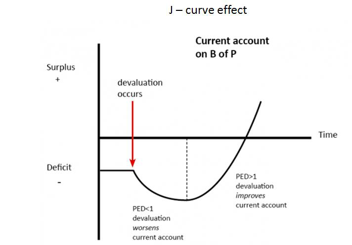
Source: Dornbush and Fisher

This phenomenon is explained by:

I. Currency Contract Analysis: Deals with the brief period immediately following devaluation (or depreciation) in which contracts were negotiated prior to the change falls due.

II. Pass Through Analysis: Deals with the behaviour of international prices on contracts agreed upon after the devaluation has taken place, but before it has effected significant changes in quantities. This article aims to compare the relevance of the Marshall-Lerner condition and the J-Curve phenomenon as the drivers of gains through the manipulation of the currency exchange rates, for the countries indulging in international trade.

The analysis included 3 type of economies (Developed, Developing and LDCs); and a total of 6 countries (2 countries each for each type of economy).

• Developed countries: USA and Japan
• Developing countries: India and Indonesia
• Least Developed Countries (LDCs): Bangladesh and Ethiopia

Results from Econometric Analysis

The results of the econometric analysis empirically established that for the Developed and Developing countries there exists a positive statistically significant relationship at 1%, between Exchange Rate Devaluation (Or depreciation) and BOT and for the LDCs, there exists a negative but statistically significant relationship at 1%. The analysis also reflected that the intensity of the positive beta coefficient was the highest for the developed nations followed by the developing and the LDCs in that order.

Also, the intensity of the Beta coefficient can be observed to be the highest on the positive side for the developed countries and highest on the negative side for the LDCs, proving that the developed countries are the ones that will reap the most benefits out of an exchange rate devaluation and the LDCs will be at the most loss. Such findings indicate that actually the concept of J-Curve is Pro-Developed nations and that can also be corroborated through the Marshall-Lerner Index of Elasticities and the level of integration of these economies in the Global Value Chain.

Also, it is observed that the developed countries are primarily exporting products that are highly sophisticated and high in value. The elasticity of the majority exports and imports is greater than 1 (>1); whereas in the case of the developing and LDC economies, the nature of import and export basket is primarily low value, intermediate goods, having lesser elasticity (<1).

It can be corroborated with trade data, that the major commodities in the import and export baskets of the developed countries lie in the upstream value chain, which is high value, technical and largely involves sophisticated final products. On the other hand the major commodities in the import and export baskets of the developing countries and LDCs lie in the downstream value chain, i.e. lower value addition, intermediate and raw goods. The Marshall–Lerner condition states that elasticities (in absolute value) must sum to greater than one for a devaluation to be effective in improving a country’s trade balance i.e. EXPORTS_ped + IMPORTS_ped > 1.

Thus, the above observation again emphasises on the fact that the Developed countries stand a greater chance of reaping the benefits from a depreciation of the exchange rate in terms of BOT surplus in comparison to the developing or the LDCs as the Exports_Ped + Imports_Ped for developed countries will be >1 at most times by virtue of the mere import and export basket that they have.

Exchange Rate of INR Vs USD

India’s Balance of Trade

We can observe a depreciation in the INR/USD exchange rate from 2005-Q1-2007-Q2. The lagged impact of this can be seen on the trade balance forming a J-Curve from 2009-Q3-2010-Q4. Another depreciation can be observed 2014-Q2 – 2016-Q1; and the lagged impact of the decline (forming J-Curve) can be observed in the trade balance from 2015-Q1 – 2016-Q2. This observation empirically testifies the visual existence of the J-Curve phenomenon in case of a developing economy such as India but the curvature is not steep as it is in general for developed nations like USA and Japan.

The findings have been able to empirically validate the existence of a statistically significant relationship between the devaluation/depreciation of foreign exchange rate and Balance of Trade. It was found that though there is a significant relationship between the two variables, but the intensity and direction of this relationship varies from economy to economy. It was also seen that the J-Curve phenomenon is highly country specific and cannot be generalised as a tool for correcting the BOT imbalances, as J-Curve reflects differently in different type of economies. With respect to the different type of economies (developed, developing and LDCs); It was observed through various types of analysis that the J-Curve phenomenon is a ‘Pro-developed’ country kind of a phenomenon.

To comment on the relevance of the J-Curve in the current global scenario, it can be conclusively stated that it is skewed in favour of the developed nations and its relevance remains limited for the developing countries and the LDCs. Though by means of a greater integration in the Global Value Chain these nations can also reap substantial benefits from overall international trade.